Ansys Mechanical Fracture Mechanics

Ansys Mechanical Fracture Mechanics

Ansys Mechanical Fracture Mechanics

one-day course

Fracture mechanics allows engineers to analyze the integrity of a structural component, where traditional methods of stress analysis are not applicable. Cracks are sharp corners, and traditional finite element analysis does not provide accurate stress at a sharp corner, also known as a singularity. The primary questions engineers are trying to answer when performing a fracture analysis are:

  • Will a crack grow under these loading conditions?

  • Where will the crack grow?

  • How long will it take for a crack to grow until the part breaks?

This 1-day course will give attendees experience in setting up, solving and post-processing finite element models with cracks in structural components. Information, such as Stress Intensity Factors, SMART (Separating, Morphing and Adaptive Remeshing Technology) crack growth and techniques for creating cracks in the finite element model will be covered.

Prerequisites for this course are DRD’s Introduction to SpaceClaim for Mechanical and Introduction to Ansys Mechanical courses. DRD recommends that students who do not have these prerequisites delay attending the course until they attain them. This is a challenging course for proficient users.

Chapter 1 – An Overview of Fracture Mechanics in Ansys

Workshop 1: Ansys Stress Intensity Factor Solution with a Simple Edge Crack ModelFracture_ws1_graphic.png

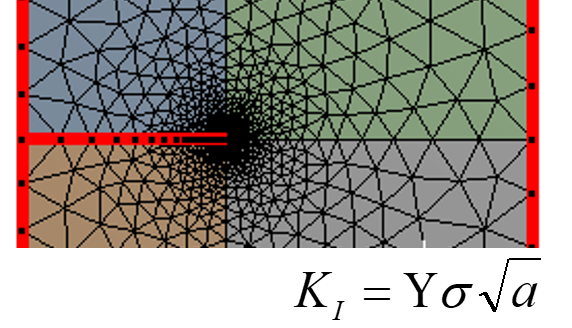
The objective of this workshop is to provide a simple basis for modeling cracks in Ansys Mechanical. The students start with a 2D plate structure and create an edge crack with the Pre-Meshed Crack capability. The student will then post-process fracture parameters, such as Stress Intensity Factor (SIF), and compare the output with a closed form solution found in many elementary fracture mechanics’ text.

The student is also introduced to residual strength curves, from both the fracture failure mode and the limit load failure mode. These curves help determine the first mode of failure for the structure.

Workshop 2: Calculation of Stress Intensity Factor at an Elliptical CrackFracture_ws2_graphic.png

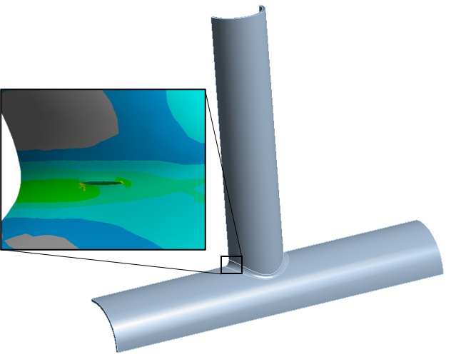
This workshop expands on the basic setup and output of the previous workshop, into a 3D model. Here, a welded pipe joint is subjected to pressure with a crack on the exterior of the pipe wall. The student will learn how to create an elliptical (or penny)-shaped crack without any prior geometry modification.

3D contours of Stress Intensity Factor are calculated for the initial case of crack size. Then, the student will modify the crack size definition, rerun the model, and compare the two solutions.

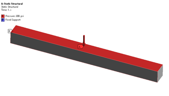
Workshop 3: Edge Cracked Plate VCCT Fracture Mechanics with Closed Form SolutionFracture_ws3_graphic (002).png

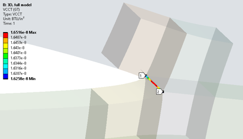
Like workshop 1, the objective of this workshop is to setup and solve a simple 3D edge cracked plate model under modeI loading. In this instance, the student will use the Virtual Crack Closure Technique. Also known as MCCI (Modified Crack Closure Integral), this method calculates a Strain Energy Release Rate (SERR) for the fracture parameter.

Students will then compare this with a closed form solution, as well as experiment with calculating a Stress Intensity Factor using Irwin’s equation.

Workshop 4: Calculation of Stress Intensity Factor and Energy Release Rate for a Double Cantilever Beam

Workshop 5: ANSYS VCCT Solution of a 4-Point Bend TestFracture_ws4-5_graphic (002).png

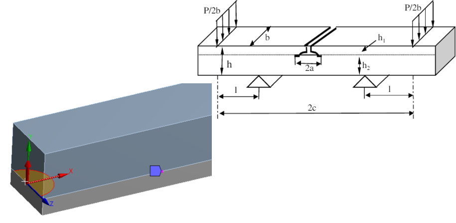
Workshops 4 and 5 demonstrate other cases of setting up and solving simple stationary crack models in Ansys Mechanical. Workshop 4 has the student setup a double cantilever beam structure. Workshop 5 uses a 4-point bend structure. Both cases have simple closed form solutions to compare to that allow validation of Ansys fracture results with known solutions.

Chapter 2 – Model Crack Growth in Ansys

Workshop 6: Computing Crack Growth with ANSYS SIFs and the Paris Law on a 2D Pressure VesselFracture_ws6_graphic (002).png

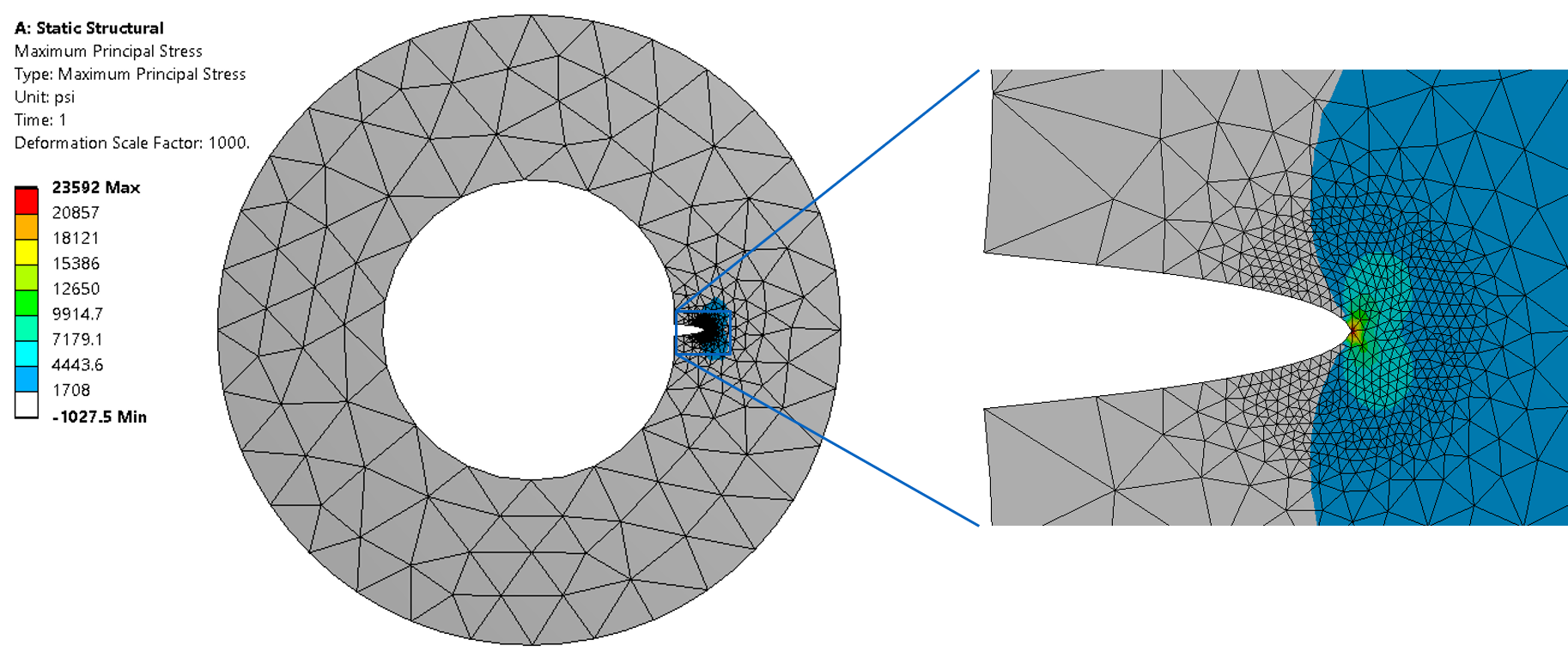
The objective of this workshop is to provide the groundwork for crack growth analysis. In this workshop, students solve a 2D pressure vessel study for varying crack lengths using Ansys Mechanical with a parametric model.

The workshop then provides a basis for computing crack growth information using a spreadsheet, allows the student to experiment with the crack growth computation, and asks several engineering questions:

·         What crack length causes immediate fracture?
·         Is limit load exceeded?
·         Is the curve fit for crack growth adequate for small cracks?


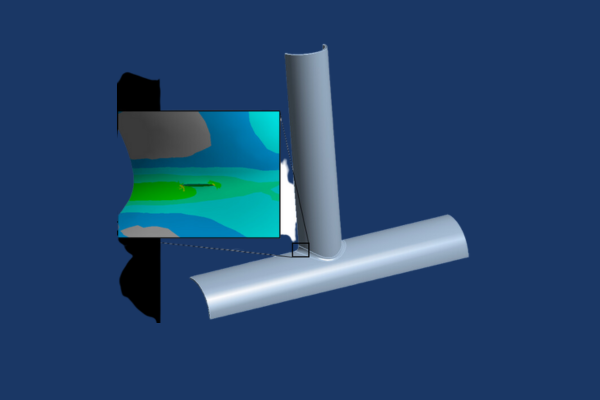
Workshop 7: SMART Crack Growth on Intersecting Pipes04292021_Fracture Mechanics.gif

This workshop is the first of two workshops that demonstrate the use of SMART. Students will learn how to setup an automated crack growth analysis using the Semi-Elliptical Crack combined with SMART Crack Growth object. Detailed definition of the Paris Law material constants for crack growth is also covered.

Automated crack growth has a host of new results post-processing options for Crack Extension, Equivalent Stress Intensity Range and Cycles; students will work through these options as well.


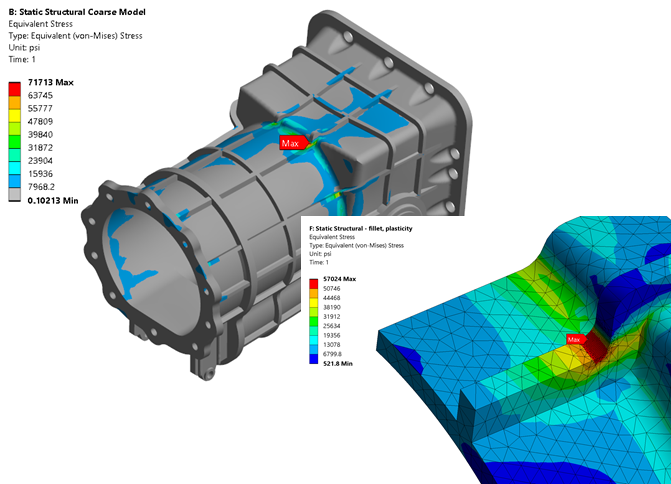
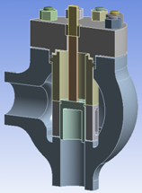
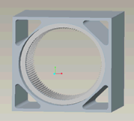
Workshop 8: SMART Crack Growth on a Casting with a Thermal GradientFracture Mechanics Training.png

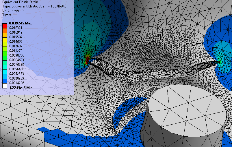
In this workshop, students learn how to create a crack using a 3D surface representation of the crack surface. This is made possible via the Arbitrary Crack feature, which allows a complex, non-planar 3D surface to be used as a basis for generating a crack mesh.


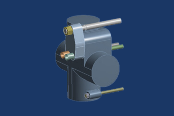
Workshop 9: SMART Crack Growth on a Casting with an Initial Stress State

This workshop is a continuation of workshop 8, where students load a casting with a thermal gradient and grow a crack. In this workshop, an initial stress state is set up that includes this thermal gradient and bolt pretension. The initial stress state is passed to a downstream analysis where the cyclic load to grow the crack is pressure. SMART crack growth is used here; Ansys automatically handles this initial stress state each time the crack calculation is performed.

Chapter 3 – Modeling Adhesive Failure

Workshop 10: Adhesive Failure Modeling with Contact Debonding

This workshop demonstrates modeling failure of an adhesive layer via bonded contact. Students define a cohesive zone material model with properties for maximum normal stress and critical fracture energy. The benefit of this capability is that the adhesive layer does not need to be directly modeled. This is a huge benefit as the adhesive layer is typically much smaller in thickness compared to the parent parts bonded together. A secondary benefit is the mesh does not need to be the same on either side of the interface, as contact is used to initial tie the parent parts together.


Workshop 11: Adhesive Failure Modeling with Interface Delamination

This workshop demonstrates a second method to simulate interface failure; interface delamination. A similar material model is defined for this method. However, contact is not required for this capability. Instead, the mesh on both parent parts must be the same at the interface with the adhesive. This is accomplished through clever meshing or match mesh controls. The interface delamination capability also has another special use case: delamination modeling with composite models created in Ansys Composite PrepPost.

Course Enrollment and Schedule

Ansys Mechanical Fracture Mechanics

Ansys Mechanical Structural Dynamics

Ansys Mechanical Structural Dynamics

Ansys Mechanical Structural Dynamics

two-day course

The objective of this course is for attendees to develop significant expertise in the use of Ansys Mechanical for dynamic analysis over a wide range of applications. The course emphasizes linear dynamic analysis, although it has one chapter and several workshops on nonlinear transient dynamic analysis. DRD collaborated with one of its customers, a large defense electronics firm, to develop important components of  this course, and most of the workshops  are practical examples based on problems that DRD has solved for its customers on a consulting basis or through Ansys technical support.

The course emphasizes good Ansys modeling practices and verification of correct solutions. DRD recommends using closed form equations based on solutions to single degree of freedom models to verify solutions to complex multiple degree of freedom models, and in this course students use hand calculations to check solutions to normal models, random vibration, response spectrum, and half sine shock models.

The course includes more than a dozen workshops in which the students use techniques covered in the course lectures  to solve real-world problems. Some of the workshops have minimal instruction so that students can begin testing their skills under the supervision of an instructor during the course.

Prerequisites for this course are DRD’s Introduction to Mechanical course and some practical experience using Ansys Mechanical. This is a challenging course for proficient users.

Chapter 1 Normal Modes (Natural Frequency) Analysis

Workshop 1a Normal Modes Analysis of an Alternator BracketStructural WS1a.gif

This bracket connects an alternator to a marine engine. The student learns to set up, solve and post process a normal modes model. The workshop involves representing the alternator as a point mass including mass moments of inertia. The student experiments with rigid and deformable connections of the point mass to the bracket attach locations. Students also learn the process of using a static solution to pre-stress the modal model and to evaluate the influence of the pre-stress on the normal mode frequencies and mode shapes.


Workshop 1b Normal Modes Analysis of a PWB Assembly
Structural WS1b.gif

This PWB assembly is representative of electronics products that many Ansys customers qualify by putting on a shaker table. This workshop reinforces skills the student began to develop in Workshop 1a. The student also experiments with the direct and iterative solvers to determine which is faster. The workshop also guides the student on how to simplify the model to a single degree of freedom systems and to check the first natural frequency with a hand calculation based on the equation f = √(K/M), where f is natural frequency, K is stiffness, and M is mass.

Chapter 2 Random Vibration Analysis

Workshop 2 Random Vibration Analysis of a PWB Assembly

This workshop extends workshop 1b to include random vibration and fatigue life prediction for a 2 hour shaker table test.  The student defines a random vibration PSD spectrum, solves the model, reviews standard deviation of stress (1s, 2s, and 3s) and finally evaluates fatigue life using the Steinberg method. Postprocessing also includes defining probes for response PSD and calculation of apparent frequency. The instructor will review the Steinberg calculations in a spreadsheet and confirm that the spreadsheet calculations match the Ansys results.

The workshop also shows the student how to approximate the 1s displacements with a hand calculation using the equation:

a = √ (Π/2 P fn Q)*
a = Acceleration in G
P = PSD value in G2/Hz from PSD curve at the natural frequency  of the SDOF system
fn = Natural frequency of SDOF system, Hz
Q = Transmissibility of SDOF system = 1/2x**; where x is the damping ratio.      


Chapter 3 Response Spectrum Analysis

Workshop 3a Response Spectrum Analysis of a Telecommunication Rack Subjected to Zone 4 Seismic Load (Telcordia Specifications)Workshop3a.png

This workshop introduces the student to response spectrum analysis in Ansys. The student will first perform normal modes analysis on a telecommunications equipment rack and then define a Zone 4 response spectrum load. Zone 4 is accepted throughout the telecommunications industry as the most severe type of seismic loading, and many companies are required to pass a Zone 4 shaker table test in order to qualify their equipment. After performing the solution with the Zone 4 spectrum the student will review the maximum displacements and stresses due to the Zone 4 test.

The workshop also shows the student how to approximate the maximum rack displacements by approximating the model as a single degree of freedom spring-mass system.

Workshop 3b Response Spectrum Analysis of a PWB Assemblywk4aa.png

This work reinforces skills the student learned in Workshop 3a. In addition the workshop guides the student through the process of making sure he uses a sufficient number of modes in the normal modes analysis to get good answers in the response spectrum analysis.

Chapter 4 Full Transient Dynamic Analysis

Workshop 4 Full Transient Dynamic Analysis of a Black Box Electronics Assembly Subjected to a Half Sine Shock

Structural WS4a.gifMany Ansys customers qualify their products by putting them on a shaker table and subjecting them to half sine shock. This workshop guides the student through a half sine shock analysis of a Black Box Electronics Assembly using the full transient Ansys solver.

The student solves the model as linear and then solves it as nonlinear by activating large deflection effects. Finally the student compares solution times and results to weigh the trade offs in modeling the structure as linear and nonlinear.

Chapter 5 Mode Superposition Transient Analysis

Workshop 5a  Mode Superposition Transient Analysis of a Black Box Electronics Assembly Subjected to a Half Sine Shockworkshop5a1.jpg

In this workshop the student solves the model of workshop 4a using the mode superposition transient solver instead of the full transient solver.

The student acquires additional postprocessing skill related to transient analysis. He also solves the model using different numbers of modes to confirm that he has used a sufficient number of modes to get good transient results.

 
Workshop 5b Seismic Mode Superposition Transient and Response Spectrum
Analysis of a Telecommunications Rack

The student subjects the telecommunications rack from a previous workshop to seismic loads from the famousStructural WS5b.gif                                    1940 earthquake of El Centro, CA. The student solves the model using the ground motion acceleration time history in a mode superposition transient analysis and then solve the same model using the corresponding response spectrum.

The student confirms that the response spectrum model stresses and displacements match the worst stresses and displacements from the transient model.

Chapter 6 Dynamic Shock Analysis using Dynamic Load Factor

Workshop 6 Analysis of a PWB Assembly Subjected to Half Sine Shock Using Dynamic Load FactorWS6_DLF#2 (002).gif

In this workshop the student uses the Dynamic Load Factor approach to solve the problem of a PWB assembly subjected to half sine shock. The DLF approach allows the engineer to avoid performing a transient solution. The DLF method involves doing a normal modes analysis and then finding a factor based on the ratio first mode’s period to the shock pulse time. The student then uses this ratio in a look up table to scale the results of a static model.

Chapter 7 Nonlinear Transient Analysis

Workshop 7a Drop Test Simulation of a Radio Housing AssemblyWS7aAnimation (002).gif

This workshop involves drop test simulation of a plastic radio housing, and it reinforces the skills the student learned in Workshop 7a. A new twist is that the student will set up an initial velocity initial condition for the housing to specify the housing velocity immediately prior to impact. The initial velocity is based on the drop height.


Workshop 7b Nonlinear Transient Dynamic Analysis to Simulation PWB Bench TestWS7b Animation.gif

This workshop introduces the student to nonlinear transient dynamic analysis. With this model the student simulates a technician’s accidental drop of a PCB on a workshop table. The model involves solving the model initially as static to set up initial conditions.


Workshop 7c Plucking Technique to Estimate the Natural Frequency of a Propeller Roof Fan Assembly

This workshop demonstrates the technique to calculate natural frequency for a nonlinear system. This fan blade assembly has nonlinear contact, and sheet metal deflections are sufficient large that large deflection effects need to be active.

The technique is a plucking technique. The first step of the solution is to perform a static analysis with imposed nonzero displacements, i.e. the pluck. In step 2 the imposed displacements are removed and dynamic effects are activated so that the structure can vibrate freely as a nonlinear transient dynamic model. The student calculates natural frequency by measuring the time between displacement peaks as the structure vibrates.

Workshop 7d Explicit Dynamic Analysis Simulating an Oblique Projectile Impactoblique ProjectileWB.gif

This workshop introduces the student to nonlinear transient dynamics using the Ansys Mechanical explicit dynamics solver. The student defines material failure criteria so that the kinetic energy project is able to make a hole through the two plates during impact.


Workshop 7e Tree Grapple Rigid Body Dynamic and Flexible Nonlinear Transient Dynamic SimulationWS7eTreeGrappleStresses (002).gif

This workshop introduces joints and the rigid dynamics solver. The student defines joints for the tree grapple mechanism and checks the system kinematic model number of degrees of freedom using  Ansys redundancy analysis. He then runs the solution with all of the parts defined as rigid using the rigid dynamics solver. The rigid dynamics solution allows the engineer to confirm that the joints are defined properly, and it also allows the engineer to check joint forces. Finally, the student makes the boom flexible, solves the model using the flexible body nonlinear transient dynamics solver, and compares the rigid and flexible body solutions.


Workshop 7f Tree Grapple Rigid Dynamic with Component Mode Synthesis SimulationWS7fTreeGrappleStresses (002).gif

Workshop 7f is a continuation of workshop 7e. The student returns to the rigid dynamics version of the tree grapple model and employs component mode synthesis (CMS) to the boom of the rigid dynamics model.  CMS allows flexible parts in rigid dynamics solutions. Finally the student compares the rigid dynamic with CMS solution to the flexible body nonlinear transient dynamic solution.

Chapter 8 Harmonic Analysis

Workshop 8a Harmonic Response Analysis of an Engine Alternator BracketWS8aAnimation.gif

In this workshop we return to the first workshop of the course, the marine engine alternator bracket, in which we calculated natural frequencies and mode shapes. We shake the bracket at its attach points to the engine with harmonic base motion acceleration, and we calculate stresses and fatigue life based on dwelling at the first natural frequency.

Workshop 8b Harmonic Analysis of a Flight Simulator Tilt Base StructureStructural WS8b.gif

This workshops involves modeling of a fuselage flight trainer tilt base. The structure has scissor mechanisms that allow 3 degrees of freedom in a kinematic sense: vertical motion, pitch, and roll. Three hydraulic cylinders provide motion and can be used to shake the structure to simulate fight turbulence. This workshop allows the student to specify harmonic motion at the hydraulic jacks that are out of phase with one another.


Workshop 8c — Rotating Unbalance Loads on a Steel StructureRotating Unbalance.gif

This steel structure has a machine on its deck that has a rotating unbalance load. We use a pair of harmonic loads 90 degrees out of phase with one another to simulate the rotating unbalance load. The model produces displacements and stresses as the structure vibrates due to the rotating unbalance load.

Course Enrollment and Schedule

Ansys Mechanical Structural Dynamics

Ansys Mechanical Nonlinear Structural Simulation

Ansys Mechanical Nonlinear Structural Simulation

Ansys Mechanical Nonlinear Structural Simulation

two-day course

This course provides an introduction to the Ansys Mechanical Environment of the Ansys software product suite.

The course focuses on use of the Mechanical user interface, which is included in Ansys Mechanical Pro, Ansys Mechanical Premium, and Ansys Mechanical Enterprise. Within this interface you read CAD geometry, assign material properties, apply loads and boundary conditions, define mesh controls, perform solutions, review analysis results, and generate an automatic html report.

The course devotes some time to theory and concepts at a very basic and practical level. These topics include finite element concepts, solutions of simultaneous equations, and contact models. These portions of the course emphasize practical theory concepts, which engineers need to understand in order to do finite element analysis.

Course requirements:

Ansys Version used to create course content: 2024 R2
Ansys Version DRD instructor will use for the course: 2024 R2
Ansys Version(s) students may use for the course: 2024 R2

Registration for all classes will close 5 business days in advance of the class date. 

Learn more: Agenda + Course Description

Chapter 1 Introduction to Structural Nonlinear Analysis and Geometric Nonlinearities

Workshop 1 3D Large Deflection Analysis of a Roto-Molded Plastic Gas Tank

This workshop provides the opportunity for the student to solve the problem first as linear and then with nonlinear large deflection effects to compare the solutions. Students also use this workshop to gain an understanding of step, substeps, and equilibrium iterations and how to use automatic time stepping.

Chapter 2a Introduction to Nonlinear Contact

Workshop 2a – Nonlinear Contact Analysis of a Ring Gear and Housing Assembly with Interference

ws2b_1.gifThis model involves calculating stresses in the housing and ring gear due to initial interference. The initial interference in combination with friction holds the ring gear securely in the housing. This workshop provides additional practice on setting up, solving, and postprocessing nonlinear contact problems.

Chapter 2b Nonlinear Contact Deep Dive

Workshop 2b – Nonlinear Contact Analysis of a Cell Phone Antenna Snap Fit 

The problem initially does not converge, and the student adjusts nonlinear model parameters to make it converge. The model then gives incorrect answers, and the student resolves that problem. The student also uses a commands object to control whether the symmetric or unsymmetric solver is used in order to improve solution performance. In this workshop the student uses a nonlinear contact solution with friction to simulate a cell phone antenna snap fit problem.   

Chapter 3 Plasticity

Workshop 3a – Nonlinear Contact Analysis of a Ring Gear and Housing Assembly with Plasticitywk4.png

This model involves calculating stresses in the housing and ring gear due to initial interference. This model expands upon workshop 2b and introduces plasticity to the model. Students post-process total strain to determine if the interference specification satisfies the design criteria of maximum 1% total strain.

Workshop 3b – 2D Plasticity Analysis of a Threaded Connection including Nonlinear Contact and Elastic-Plastic Behavior

This model represents a four part threaded connection assembly. Nonlinear contact is used to model interaction of the threads and the mating surfaces of the other parts. Students define a multilinear elastic-plastic model and calculate plastic and total strains.

Chapter 4 Eigenvalue and Nonlinear Buckling

Workshop 4a – Linear and Nonlinear Buckling Analysis of a Steel Columnnew_anim (002).gif

This assembly is a C-channel shaped column with a cap and a base, all composed of A36 steel. A downward vertical load is applied at the top of the column that will cause it to buckle. DRD introduces the methodology of solving a buckling problem: from a simple Eigenvalue, or linear buckling analysis to a nonlinear buckling analysis where an elastic-plastic material model is employed to simulate permanent deflection and local instability. Students will learn the workflow analysts typically use to solve buckling problems.

Workshop 4b – Snap Through Analysis of a Spherical Tank Section Using Stabilization03022021_Nonlinear 2.gif

A section of a curved tank needs to be analyzed to check deflections and stress. This geometry will buckle when a sufficient load magnitude is applied. Solution restarts and the stabilization feature is utilized in this workshop.

Chapter 5 Hyperelasticity

Workshop 5a – 2D Axisymmetric Analysis of a Hyperelastic Rubber Seal with Nonlinear ContactDRD Workshops0002.png

This four part assembly model has two rubber parts modeled using a hyperelastic material model. Students import experimental data into the Workbench Engineering Data module and curve fit it to create Mooney-Rivlin constants. Initially the model does not converge, and students must modify the model to get it to converge. The model also provides an opportunity for students to experiment with different nonlinear contact formulations including pure penalty, augmented Lagrange, and normal Lagrange.

Workshop 5b – 2D Axisymmetric Analysis of a Hyperelastic O-ring with Fluid Pressure Penetration Loading

This model is comprised of three parts – a cylinder, ring, and seal. The cylinder enters the bore and contacts the seal to produce pressure between the cylinder and ring. Ideally this pressure would be great enough to keep fluids from breaking the seal. The second step applies fluid pressure to the exposed portion of the seal and continues to be applied to the portions of the seal that ‘peel away’ from the cylinder or ring. This fluid pressure penetration capability in Ansys is critical in determining seal performance.

Workshop 5c – 2D Axisymmetric Analysis of a Hyperelastic O-ring with Nonlinear Contact, Using Nonlinear Adaptive Remeshing (NLAD)

This model contains a tube, sleeve, o-ring and swaging body. The swaging body is pushed down, causing the tube 
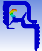
to be plastically deformed into the seal, which is a hyperelastic body. A pressure is applied to the inside of the tube at a subsequent time. The o-ring undergoes severe deformation; the Nonlinear Adaptive Remeshing technique is used to remesh the model during the solve process automatically to get a completed solution, rather than the user remeshing manually if the model fails to solve.

Chapter 6 Bolt Pretension

Workshop 6a – Nonlinear Contact Analysis of Steel Enclosure with Bolt Pretension

This four part assembly is held together with a pretensioned bolt. Students use Simulation bolt pretension to load the model. The objective of the model is for students to gain a thorough understanding of Simulation bolt pretension. This model also provides additional practice in modeling nonlinear contact.

Workshop 6b – Analysis of a Pump Fluid End with Bolt Pretension

This pump assembly is held together with four pretensioned bolts. Students use load steps to sequentially pretension the bolts one step at a time and then apply additional loads.

Chapter 7 Submodeling

Workshop 7 – Stress Analysis of Gearbox Casing Subjected to Static Loads including PlasticityNonlinear WS 6.png

This gearbox casing is subjected to force and torque loading and the objective is to determine peak stresses in the structure. Students will use the submodeling process, which is based on St. Venant’s Principle, to build a coarse-grid model, take the displacements from locations within the coarse-grid model and apply them to a fine-grid model boundaries. Use of plasticity will be required to get accurate stress beyond the yield strength of the material.

Ansys SpaceClaim will be used to create the fine-grid model using the coarse-grid model as input.

Chapter 8 Gasket Modeling

Workshop 8 – Nonlinear Contact Analysis of a Control Valve including Gasket Behavior

This control valve has two gaskets, and the objective of the analysis is to optimize the gasket design. Workbench does not yet have gasket elements, so students use DRD developed commands objects to add gasket elements to the model. The model also involves bolt pretension, pressure, mechanism forces, and thermal loads. The model requires linear and nonlinear contact types. Students define temperature dependent material properties.

The initial design does not have a viable gasket design, and students use a design parameter and DesignModeler to modify the design to achieve an optimum gasket design.

Appendices
Workshop A – Nonlinear Contact Model for Insertion and Removal of a Mechanical Connector
Students solve this mechanical connector problem using nonlinear contact with friction. Weak springs prevent rigid body motion at the beginning of the solution.  The course materials provide only a general description of the problem and objectives, and students must solve the problem without detailed instructions.

Workshop B – Nonlinear Contact of a Swaging Operation including Elastic-Plastic Behavior

Students simulate the swaging operation using nonlinear contact with friction, a bilinear elastic-plastic model, and a multilinear elastic plastic model. This workshop requires conversion of a stress-total strain curve to a stress-plastic strain curve for defining the multilinear plasticity model in the Workbench Engineering Data module. The course materials provide only a general description of the problem and objectives, and students must solve the problem without detailed instructions.

Workshop C – Shell Model for a Battery Clip including Nonlinear Contact and Plasticity

This model involves modeling of nonlinear contact and plasticity in a structural shell model. The model simulates the compression of the spring when a battery is inserted into an electronics device. Students modify the nonlinear contact definition to account for shell thickness effect, and determine its effect on the strain in the clip.


Workshop D – Nonlinear Contact Model for Insertion and Removal of a 3D Mechanical Connector

This model is a 2-part mechanical connecter. The spring leg is inserted into the chassis and then removed. The main goal of this analysis is find out the force required to insert the spring leg into the chassis and then remove it from the chassis. It is also desired to find out the resulting stresses in the connector due to insertion and removal.


Workshop E – Large Deflection Analysis of a Cantilever Beam using Restarts03022021_NonLinear_WS E.png

The main objective of the workshop is to calculate the stresses and deflections of the beam under a given loading. The workshop will stop and start using the restart capabilities of Workbench. Additionally, APDL post-processing commands will be inserted and executed without re-solving the model.


Workshop F: Hyperelastic Model with Nonflowing Incompressible Fluid

This model is comprised of three parts – top and bottom plates and a rubber fluid bladder. The bladder is compressed and non-flowing fluid elements are placed in the bladder to maintain a zero volume loss. Students use MAPDL commands to define the hydrostatic fluid elements HSFLD242 to simulate this non-flowing fluid in the bladder. The resulting force deflection curve is obtained.

Course Enrollment and Schedule

Ansys Mechanical Nonlinear Structural Simulation