Occasionally it may be a requirement to report average values of stress or strain from an ANSYS Mechanical analysis. There are tricks to do this either for a group of nodes/elements on a face or elements within a specific volume.

Depending on the requirement, the goal may be to simply report either :

– “Average” stresses on a face (based on nodes)
– “Average” stresses on a face (based on elements)
– “Average” stresses on a volume (based on elements)

Technique 1 : Reporting weighted area average nodal stress

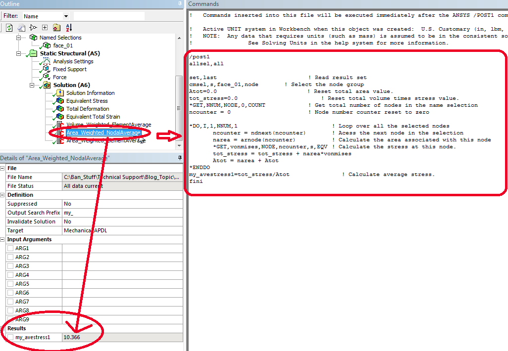
This can be done by implementing the macro in a command object as shown. The weighted area average nodal stress on the surface is reported under the details of the command (in the red circle below) with the parameter named “my_ave_stress1”.

The contents of the command object can be downloaded here.

Note: The surface chosen to do the averaging is defined as named selection ‘Face_01’ (used in the macro). In this technique the weighted averaging is done by calculating area apportioned to the nodes, and multiplied with the corresponding stress values for those nodes, and then summed up, and then we divide that sum by total area of nodes.

Technique 2 : Reporting weighted volume or area average element stress

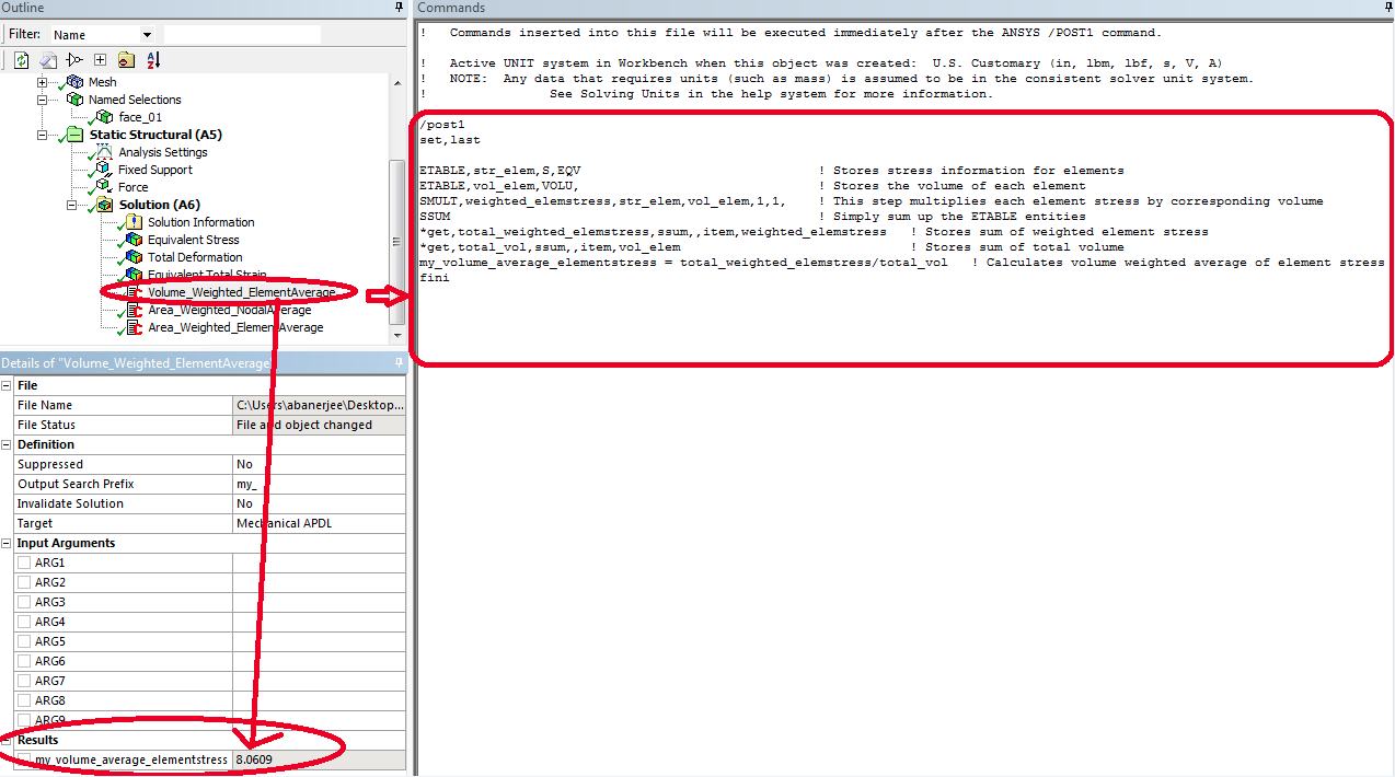
DRD recommends doing element averaging that is weighted based on volume. This can be done with a command object (shown below) and you can download it here.

If the goal is to use the element area to do the averaging, then there is a technique for this as well. This method is written for 3d solid elements belonging to the ANSYS 18x series solid elements such as : 185 (dropped midside node bricks), 186 (20 node bricks), 187 (10 node tets).

In this technique, you define the surface using a named selection (Face_01). You will additionally create a remote point referenced to that named selection. This is a clever trick, since in a solid 3d mesh, it is not directly possible to know the area of the element face easily. By creating a remote point, we are creating contact/target elements which are then tagged to the solid elements overlaid on that surface, and the area of contacts gives us the area of the solid element faces which can then be used for the element averaging.

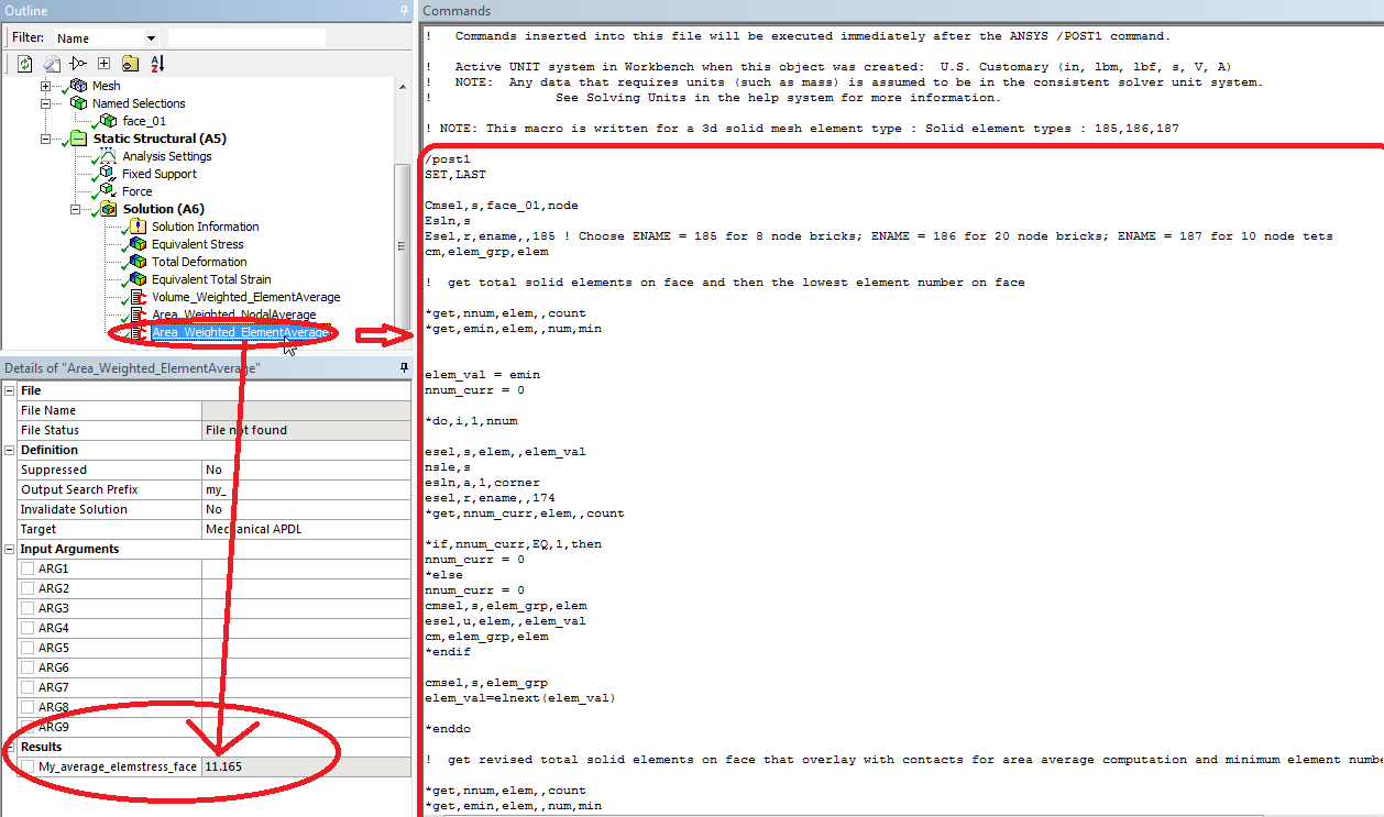
This can be done by implementing the command object as shown. The content of the command object can be downloaded here.

The weighted area average element stress on the surface is reported under the details of the command as shown with the parameter named “My_average_elemstress_face”.

Note: If you are running a SOLID 185, 186 or 187, you need to specify that in the command snippet as highlighted below.  In this technique, the weighted averaging is done by calculating area of the elements, multiplied with the corresponding stress values for those elements, summed up, and then we divide that sum by total area of elements.

DRD recommends you test these techniques on a simple part first before attempting on a larger model, and be sure to do the necessary sanity checks to ensure results are accurate.

Boundaries in Ansys Fluent can be broken into two groups: external boundaries and internal boundaries.  External boundaries appear on the outer boundary of meshed regions (inlets, outlets, interfaces, etc.), while internal boundaries exist within a conformal mesh (interiors, porous-jumps, fans, etc.).  Notably, internal boundaries can exist inside a single cell zone, or can even separate different cell zones as long as the mesh is conformal across the boundary. There is one boundary type that can be used as either an external or internal boundary: walls.

While external walls are straight forward, internal walls are a bit more complex. Internal walls are sometimes called coupled walls or two-sided walls because they are formed by a pair of wall boundaries that are by default coupled together. You most often see coupled walls separating fluid and solid cell zones, but they can also be used as infinitely thin baffles with fluid on both sides.  Each coupled wall pair shows up in the boundary list as a zone and its shadow: one for each side of the wall.  When the coupled wall is between two different cell zones, it is easy to determine which side faces which cell zone as the adjacent cell zone is listed in the boundary condition window.

It is possible for a two-sided wall to exist between a single cell zone. When this occurs, the above reference to the “adjacent cell zone” is no longer useful to determine which side of the wall faces a particular direction. In these instances, it is possible to plot the face area in the direction most aligned with the boundary’s normal direction. The face area vector points from the adjacent cell into the wall (this is opposite of face normal direction). Note that you must initialize the solution to be able to generate the necessary contour plot.

In the below example, the “X Face Area” is plotted on the wall-baffle-shadow zone. The plot shows that the area is largely negative, which implies that this wall faces the +X direction. While this may initially seem backwards, keep in mind that the face area points from the adjacent cell towards the wall. This is backwards of the outward facing normal direction.

Hopefully this article sheds some light on wall/wall-shadow pairs. If you require further assistance with this topic, please contact us at support@drd.com.

When setting up rotating machinery in Fluent, users will specify a rotating cell zone with the appropriate angular velocity. The bounds of this domain must be surfaces of revolution for either the frame motion or sliding mesh approaches. This article focuses on the finer details of setting up such a case. Particularly, what needs to be done for walls on the boundary of a rotating zone that should not be rotating? Additionally, sometimes a rotating shaft will exist both within a rotating zone and also within an adjacent stationary zone, how should this be handled? This article will answer these questions.

As an example, consider a case where a fan is placed within a circular duct. It is held in place via the motor and motor mounts. The domain will be split into rotating and stationary zones about halfway along the shaft that connects the fan and motor assembly.

The setup of the rotating zone itself is straightforward. For this analysis, the frame motion approach will be used.  In the Cell Zone Conditions Panel, the “Frame Motion” box will be checked and the appropriate rotation axis, rotation axis direction, and rotational velocity will be set.

In Fluent, all walls are stationary relative to their adjacent cell zone. This means walls within or on a rotating zone are rotating with that zone. Similarly all walls within or on a stationary zone are stationary. Consider the two images below. The duct in the rotating cell zone should not be rotating with the fan. Conversely, the motor shaft that extends into the stationary zone should be rotating, while the cell zone should be stationary. These conditions need to be applied at the boundary level for these two walls.

The small section of shaft in the stationary zone will be treated similarly, but will instead have the same angular velocity as the rotating zone. In this model the small section of shaft in the stationary zone likely does not change the result much, but this will not always be the case.

One very important aspect of applying wall velocities as done for both the duct and the shaft is that no velocity can be applied normal to the wall. In the case of cylindrical walls, only rotational velocity around the axis of the cylinder is allowed.

Porous media is widely used in CFD to reduce the computational expense of modeling things like filters, perforated plates, and tube banks. To accomplish this reduction in computational expense, the losses across the porous device are modeled mathematically using a simple equation rather than by geometrically resolving the flow obstruction.

Using the porous media model requires knowledge of the loss coefficients. These are referred to as the viscous and inertial loss coefficients. These coefficients can be derived from experimental data, empirical correlations in literature, or through CFD. The CFD models used to determine these coefficients are small sections of the full device, which makes the computational expense relatively small.

The pressure loss through a porous domain is represented by the following equation:

The unit cell model will be run at several flow rates and the pressure drop across the model will be recorded. The velocity vs pressure drop curve formed by this data will be curve fit to the form:

Coefficients a and b will then solved for using:

Knowing that the pressure loss will always follow a parabolic curve as described above, any tuning that is perceived to be needed means that the curve fit must be altered. Similarly, if experimental testing reveals that the pressure drop vs velocity curve follows any shape other than a parabola with a y-intercept of zero, then the porous loss model cannot represent this loss accurately across, though a curve fit could potentially be done for some limited range of velocities.

Reflecting on my Time at DRD Technology

Since I had exposure to DRD Technology at previous companies, I now have a seasoned view as a customer and as a team member of DRD Technology. Over the past 15 years, in roles including Senior Applications Engineer and now Chief Technologist, I have had the opportunity to work on some incredible projects.

First, since Ansys is a company that is constantly innovating, a large part of my job is to keep up with the latest developments and evaluate them for our team. When I see a new tool that could be useful, I evaluate it thoroughly to ensure it meets our needs and can integrate smoothly into our workflow. One focus area for me has been on a tool called HFSS, which has become a cornerstone of our company’s offerings, and my role has continued to evolve as I work to identify new Ansys technologies that enhance our company’s offerings.

In general, my role is 80 percent pre-sales work and 20 percent supporting technical questions and conducting training courses periodically. Pre-sales allows me the opportunity to work closely with the sales team in the early stages to understand the client’s needs and requirements, and then develop a solution that would meet those needs.

Over the years, I have worked on many different projects. One of the most memorable was a pre-sales project for uAvionix four years ago. uAvionix is a company that builds innovative products for aircraft many of which have integrated RF antennas and my project was to simulate one of their products as “proof-of-concept” effort. When I presented the results to the client, the output from HFSS and measured scope trace results on the same graph were practically identical! I was completely amazed at the accuracy of the simulation in this case. Most numerical simulations are good if they fall within 10 percent of measured data, but this HFSS solution was within <1% of the measured data. That was the first time I ever experienced a predictive physics simulation being that “predictive.” This specific project has always been stuck in my mind; it was quite amazing.

Today, most CAD program providers include an embedded option for conducting simulation. This option is appealing to many companies as their engineers can expand how they use the tools they already have available for low or no additional cost. For many companies, their existing CAD licenses provide a low-barrier-to-entry way to test drive simulation. As a company gets started with simulation, or if their simulation requirements will remain fairly simplistic, a CAD-embedded tool can be a great option. However, since the simulation technology included by many CAD vendors was acquired as a means to complete their product offerings, oftentimes, the level of simulation available is limited in scope and size of model and may not be a great long-term solution. 

So how do you know when you are outgrowing the capabilities of your CAD-embedded tool? Some examples of questions to ask your simulation team to determine if a CAD-embedded or standalone product is the best option for your needs include the following: 

• What are the limits to your simulation?
• Do you have large assemblies?
• Do you require advanced or coupled physics?
• When it comes to simple physics, do you have lots of parts and/or a complex model?

For a more detailed review of a few examples and additional related issues,  DRD encourages you to read our whitepaper “Six Considerations for Selecting Engineering Simulation Software”.

(link the whitepaper title to the registration page on our website to download it – https://www.drd.com/resources/engineering-simulation-software-wp/)