Troubleshooting Common Ansys Mechanical Errors: Solutions for DOF Limit, Unconverged Solutions, and Element Distortion
When solving complex models in Ansys Mechanical, several common errors may arise. In this blog, we’ll explore three frequent error scenarios—DOF limit exceeded, unconverged solutions, and element formulation errors—and provide solutions for each.
Error Scenario 1: DOF Limit Exceeded
This error indicates that at least one body in the model has reached a degree of freedom (DOF) limit, often due to rigid body motion (RBM). Mechanical will prompt you to check for insufficient constraints. This situation is typically a result of rigid body motion (RBM), and Mechanical will have a message suggesting the user search for insufficient constraints.
In a static analysis, every part in the model must be constrained so it cannot freely rotate or translate. RBM is a consequence of one or more parts being insufficiently constrained. Check that there are enough external constraints on the model (i.e. supports) to prevent RBM. Here’s how to resolve this:
- Ensure that all parts are constrained or connected to supported parts.
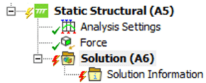
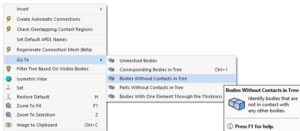
- Be attached to supported parts using contacts, joints, or other connections. Mechanical offers a right-click menu in the graphics area with an option that can identify missing connections (below).
If you are depending on nonlinear contacts (Frictionless/Frictional/Rough) to hold the model together, make sure they are initially closed. The Contact Tool is a great help for this. Be aware that nonlinear contacts will not prevent separation, and they may not prevent sliding either.
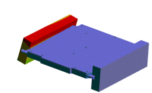
If you are not able to identify any parts that are underconstrained, try running a Modal analysis with the same supports as your static analysis. The animated deformation plots from the Modal analysis should help you identify what parts need constraints. Pay special attention to modes at 0 Hz or very close to it. The mode animation below shows one part moving without deforming the rest of the assembly, indicating that it is underconstrained. Be aware, however, that Modal analysis forces nonlinear contacts to become linear, so it may not identify all problems with nonlinear contacts.
Error Scenario 2: Unconverged Solution
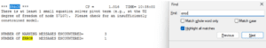
In this scenario, you may see the line “Reason for Termination … Unconverged Solution” in the solution information, and there will be an Error message in Mechanical that reads, “The solver engine was unable to converge on a solution for the nonlinear problem as constrained.”
This error occurs for nonlinear models. When a model is nonlinear, the solution affects the model’s stiffness, and the solver needs to iterate on a solution until the remaining error is within tolerance. There are three main factors that can cause a model to be nonlinear: material properties like plasticity, nonlinear contact types, and the Large Deflection option under Analysis Settings. One or more of these nonlinearities is responsible for the failure to converge. You will need to identify which nonlinearities are the cause.
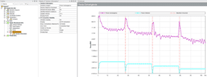
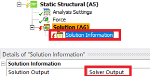
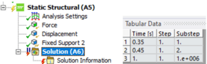
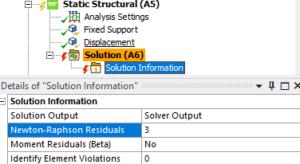
The most helpful tool for troubleshooting a force convergence error is Mechanical’s Newton-Raphson Residuals. In the Details of Solution Information, set this to some non-zero value (2 or 3 is usually enough). The plots will only be created if a non-zero value was set before the analysis was solved. You may need to initiate the solve and let it fail again in order to get the Newton-Raphson plots. Adjusting the time steps to ensure it fails quickly is recommended. Before re-attempting the solve, you may wish to try the other troubleshooting steps in this section.
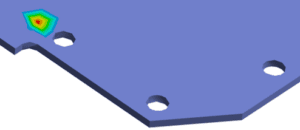
The Newton-Raphson Residual plots will show hotspots (red color) where the residuals are highest. This means you should look for conditions that are scoped to these elements. Often you will see high residuals on elements that are participating in a nonlinear contact region. If so, this contact region needs attention.
Possible solutions to a contact region with high Newton-Raphson Residuals include:
- Mesh refinement on the faces scoped in the contact region.
- Reducing normal stiffness of the contact region to a Factor of 0.1 or 0.01.
- Using a linear contact instead of a nonlinear one if acceptable.
- Using displacement-based loading rather than force-based loading to close a contact region that is initially open.
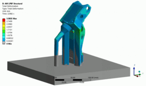
Aside from the Newton-Raphson Residual plots, there are a few other tools that can help narrow down the reason for non-convergence. Per the last section, make sure the model is fully constrained and rigid body motion is not possible. If any substeps have solved, create True Scale deformation plots for the solved time points and look for any unexpected behavior such as large deformations or assemblies separating. Plots of plastic strain can identify regions that are collapsing due to widespread yielding.
If you’ve reviewed the Newton-Raphson Residual plots and solved timesteps but it still is not clear what is causing the analysis to fail, a useful approach is to remove all nonlinearities from the model and make sure it solves. If it does, then add nonlinearities back into the model gradually. When you reintroduce a source of nonlinearity and the solve fails again, you can be confident that this nonlinearity is what needs attention before the solve can succeed.
Error Scenario 3: Element Formulation Errors
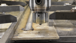
This reason for termination is often accompanied by the error message in Mechanical: “Element N Located in Body (and maybe other elements) Has Become Highly Distorted.” The element formulation error means that certain elements fail to meet criteria that are required to obtain a meaningful solution. Most often the elements have become so distorted that the analysis cannot continue. An ideal element is a cubic hexahedron or a tetrahedron with four equal sides. When elements have high aspect ratios, have highly skewed shapes, or even begin to turn inside out, they are liable to terminate the solver with this error.
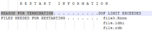
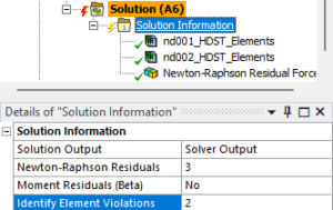
The first step is to identify the elements that have the error. Look at the error messages in Mechanical and the Solution Information worksheet for specific element numbers. Then find where these elements are located in the mesh (this video shows how; use the element option instead of the node option).
There is also an option to create Named Selections for element violations under Solution Information. Set this to a non-zero value (2 is usually fine).
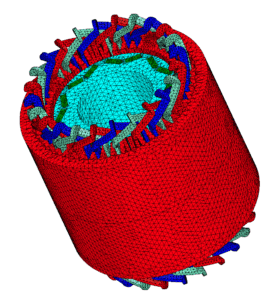
Using either the Named Selections or the Select Mesh by ID tool, observe the element shapes and locations. If they are highly skewed, it may help to improve the mesh in that area to get better quality elements.
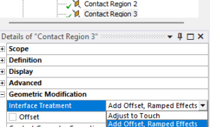
Another important step is to find out how far the solver made it before the failure occurred, as described earlier. If no substeps solved, then there was a problem applying the initial conditions. Use the Contact Tool to identify contacts that have initial penetration. If you have any nonlinear contacts with initial penetration, use the Add Offset, Ramped Effects setting for those contacts, or Adjust to Touch if you wish to ignore the penetration. Elements in contact regions can easily get distorted when the penetration is removed with the No Ramping setting.
If you do have solved substeps, use the plots of the solved substeps along with the locations of the element violations. (Note again that results set to Display Time = Last are unconverged and are not meaningful.) Are these elements starting to distort just before the failed time step? Is there a lot of plasticity on these elements? If the elements are actually becoming distorted, you may need to improve the mesh to get better initial quality. In scenarios with a lot of plasticity, you may not need to solve the whole analysis if the solved time steps already show levels of plasticity that indicate failure of the product.
Sometimes the elements do not seem to be visibly distorting in the solved time steps. In that case, they may be distorting due to a load being applied too suddenly or due to insufficient constraints. Think about whether there are new loads being applied in the time step that failed, or whether there are parts about to come into contact. Consider ramping loads more slowly or using displacements rather than forces to move parts into contact.
Nonlinear modeling in FEA is a deep subject, and not every scenario or possible solution is covered here. Even so, we hope this guide will provide a starting point that will help you solve complex models in Ansys Mechanical.
Understanding error messages is crucial, but to prevent them, identifying them is key. Don’t miss our blog on how to use Ansys Mechanical’s troubleshooting tools to resolve failed solves and produce accurate results.